After I published my article: “Bolted connections in ANSYS workbench part 1“, I was asked by several readers to write part 2. So here it is. The purpose of this post is to understand at the fundamental level:

1. How bolted joints work.
2. How simple analytical models compare with the FE models.
3. How a simple, widely used FE model of bolted joint compares with a detailed threaded contact FE model.

For this purpose, I created a simple, 2D axisymmetric FE model of a large M64 sized tension loaded connection typically found in 10MW+ wind turbines. Although, the analytical approach described here is applicable to any bolted joint application and is based largely on VDI 2230 methodology as described in the book “Introduction to the Design & Behavior of Bolted Joints” by John H. Bickford. I’ll keep things simple and the focus will be “analysis” of a given joint rather than “design”. I’ll come to designing a bolted joint in later parts of this series.

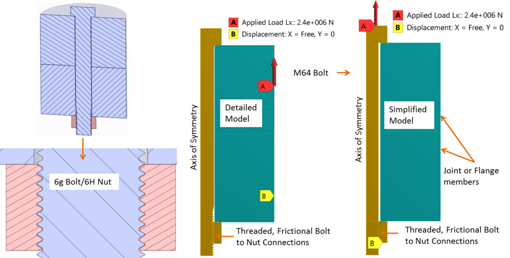
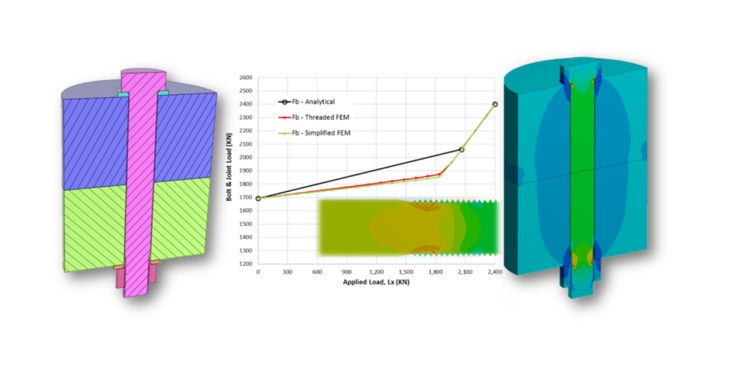
The two FEM models are shown above. In the first or detailed model, threaded frictional contact is created between the nut and bolt. Additionally, the bolt geometry is realistic and includes tapered shank before the threads as well as fillet at the bolt head to shank corner. The threads are based on 6g/6H tolerance which is applicable for general use in commercial applications such as wind turbines. Please note here that if you model the basic (ideal) thread geometry, there will not be any gap between the threads and the resulting stress distribution will not reflect reality. I also rounded sharp thread corners with small 0.3 mm radii since, in reality, no sharp corners exist and to prevent any stress singularity. The only simplification, I have with regards to geometry is that the threads do not have a helix angle in order to make use of the axisymmetry model.

The second simplified model does not include any threads. The bolt to nut connection is bonded and the bolt has a straight shank (no fillets) with a cross-sectional area equal to the tensile area of the bolt. This is typically how I create 3D or beam element bolts in my professional work.

I have used two sets of boundary conditions. In the first set, the external tensile load on the joint is applied directly to the bolt head while holding the nut. This is not how loads are applied on the joint, however, the simplest analytical model of a bolted joint is based on this assumption so I am curious to see how it compares with the FE model. In the second set of boundary conditions, the load is applied on the side of cylindrical joint members while the bottom flange (cylinder) side is held in place. This is more realistic as the load coming from the rest of the structure will get transferred to the joint via the joint members. In the future, I’ll create a more realistic model of a flange section instead of cylindrical joint members used here. However, for the purpose of what I am trying to achieve, this 2D axisymmetry model is appropriate. The two sets of boundary conditions were applied to both models.

To create 2D axisymmetric models like this in ANSYS workbench, you have to keep in mind the following points:

1. Make sure that the y-axis is the axis of symmetry and the 2D model should be created on the positive side of the x-axis.
2. For the bolt preload, create a new coordinate system with the x-axis rotated along the bolt axis whereas the y-axis is where bolt pretension section will be created. The x-axis can be located anywhere but in my models, I’ve aligned it with the axis of symmetry.
3. For applying bolt pretension select “body” instead of “face”.
4. Apply full load to the 2D section as if you are applying it to a 3D model.

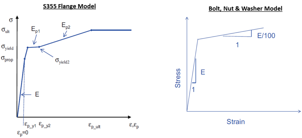
The FE material models used in this analysis are based on the DNVGL-RP-C208 guidelines. For the flange, a multilinear kinematic hardening model is used and a bilinear model is used for bolt & nut with the second slope set to 1/100th of young’s modulus E as per the guidelines. The bolt is grade 10.9 which means yield strength ~ 900 MPa and ultimate strength of 1000 MPa. The analytical model is based on linear elastic assumption. The analytical step by step hand calculations is shown below:

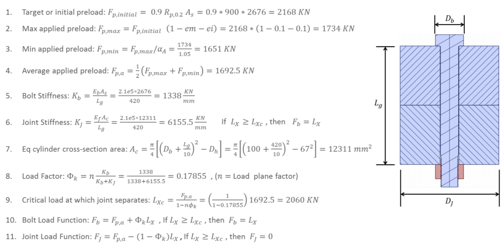
In the first step, the initial or target or the desired preload is calculated based on 90% proof strength of the bolt. In step 2, the maximum preload is computed after taking embedment relaxation and elastic interaction losses. Embedment relaxation occurs due to the microscale compression yielding of washer and joint material in contact due to initial preload. The elastic interaction loss is a result of the tightening of adjacent bolts. In this analysis, I’ve assumed a 10% loss for each for a total of 20% loss of initial preload. In step 3, the minimum preload is computed taking into account the scatter due to the particular tightening method used. For the usual wrench method, the scatter can easily be ~30% and so the value of the alpha_A parameter can be as much as 1.3. However, in this case, I am assuming just 5% scatter which is achievable in case of pre-tensioning up to yield. I am basically using 5% to keep the preload within the ~1650 KN range. In step 4, the average remaining preload is computed and this value is used in subsequent calculations. In steps 5 and 6 stiffness of bolt and joint members are computed based on the simplest formulas available. For the joint member stiffness, I’ve used the equivalent cylinder model as described in Bickford’s book. There are better but more complex models available for both the bolt and joint stiffness calculations (refer to the VDI 2230 documents).

In step 8, the load factor is computed which defines the fraction of applied load taken by the bolt vs the joint members. This parameter typically varies between 0.15-0.2. The load plane factor n determines how the load was applied. For the simple case of bolt-Nut loading, this factor is 1. For sideloading boundary condition, this factor can be as low as 0.25 but I’ve used a more conservative value of 0.5. In step 9, the critical external load is computed at which the joint separates. This is regarded as a failure of a tension joint since after separation, all the load is carried by the bolt. Finally, in steps 10 and 11, I generate the bolt & joint load functions.

In the FEM model, I follow the same process. The initial preload is applied in the first load step. In the second load step, bolt preload is relaxed to the average assembly preload value. In the third load step, external load Lx is applied.

Graphs of bolt & joint load functions are compared with FEM below. The joint load FJ is the compression of the joint (hence negative force values). As applied load Lx is increased, the joint load hits zero load line, implying joint separation. At exactly the moment when the joint load hits zero, the bolt load function changes slope which indicates that all applied load is now carried by the bolt. This ultimately leads to a fracture of the bolt but for all practical purposes, failure of the joint already happened at separation.

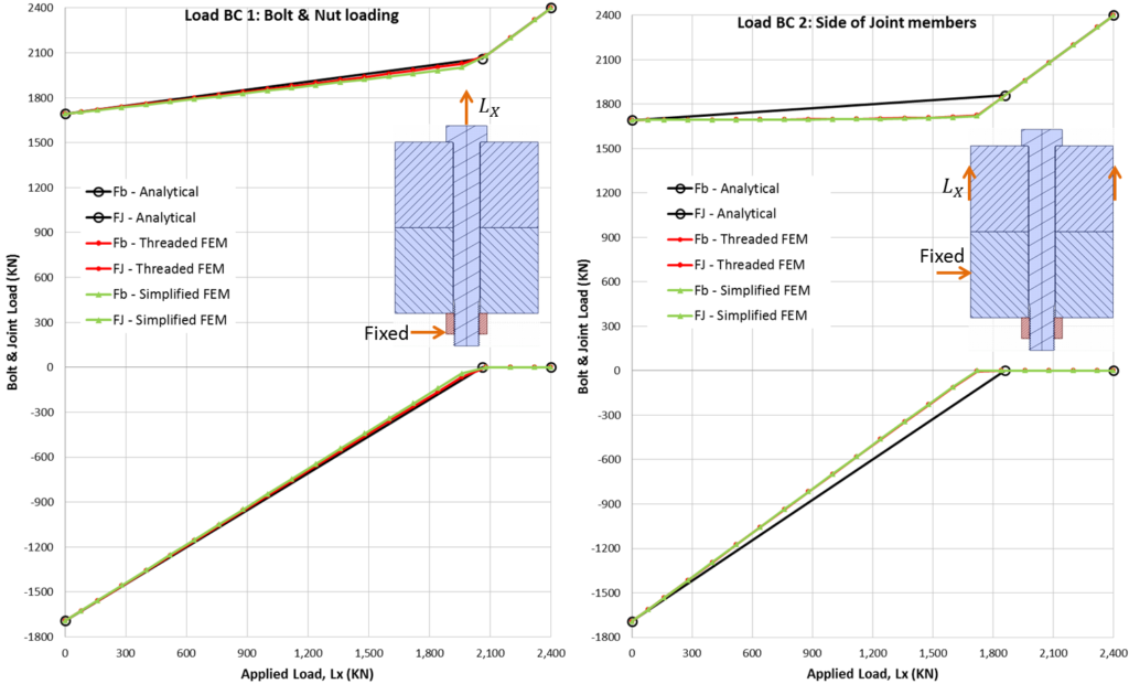
For the case of bolt loading and fixed nut boundary condition, the analytical calculations match really well with FEM models. For the second set of boundary conditions (n = 0.5), the match is not as good. In both cases, the simple and detailed FEM models match very well.

I often design joints analytically before resorting to FEM, therefore, it is of interest to see how well the analytical model compares with FEM. The analytical slope of the bolt load function is greater which is more conservative since, in the real world, we never have perfectly matching flanges as modeled in FEM. Any flange imperfection will result in an increased slope which is very critical for fatigue calculations. On the other hand, joint separation load is greater compared to FEM which makes analytical calculations less conservative but overall I think, the analytical calculations are good enough for sizing the initial joint at the preliminary design phase.

The detailed model provides some interesting bolt stress results especially around the threads as shown below at the end of load step 2 (maximum applied load).

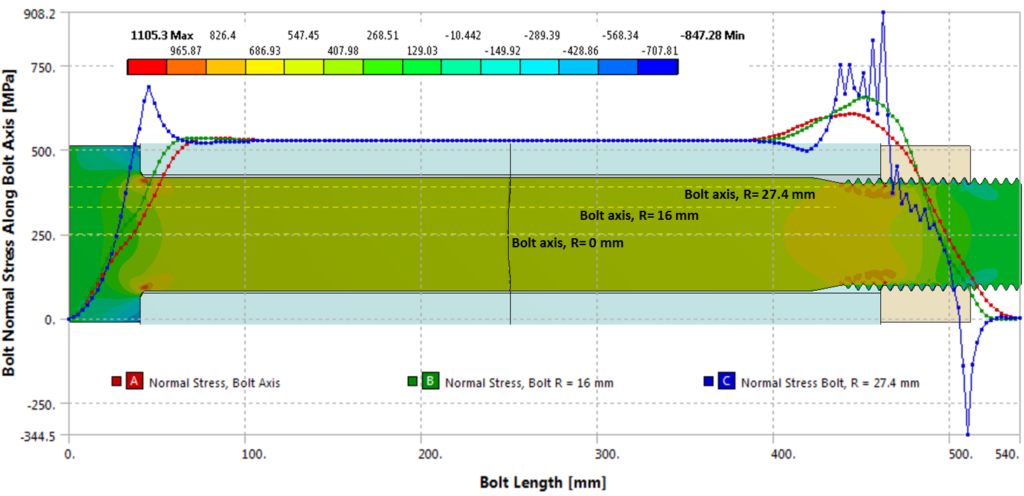
Notice, how the stress peaks in the first nut-to-bolt thread along the path line at R = 27.4 mm which passes just under the root of bolt threads. This variation of normal stress through all load steps is best viewed in an animation:

Notice how the thread stresses remain unchanged until the applied tension load causes the joint members to separate. Follow the simulation time which indicates load steps. So at time t=2.0 sec, the load is applied and joint separates at ~ 2.7 sec which means at 70% of the maximum applied load of 2400 KN. After this point, the stresses go up rapidly. This shows the importance of ensuring the bolted connection always maintains contact. Once the joint separates, it will only take a small increase in load to break the bolt due to the steeper slope.

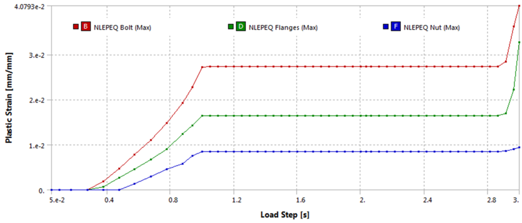
Also, notice, the stress in the bolt threads goes past yield at initial tightening (LS 1). After relaxation (LS 2), the threads become strain hardened. In the subsequent loading step, no additional yielding happens until the joint separates and the bolt takes all the load. The growth plastic strain in the bolt threads and adjoining nut and joint member can be seen here in this simulation:

The growth of plastic strains in the nut, bolt and bottom joint member can be seen in this chart:

There is a lot more we can learn from this simulation, but I’ve to end this post here and continue in part 3 of this series. In the meantime, if you have questions, please reach out to me at zaeem@endeavos.com